
PINNs, Neural Operators, and the Future of Simulation

This is part one of a two part series. This is something I’m still learning about. I’m early in my understanding here, so consider this an exploration of recent conversations with some experts in the field as well as what I’ve been reading and listening to.
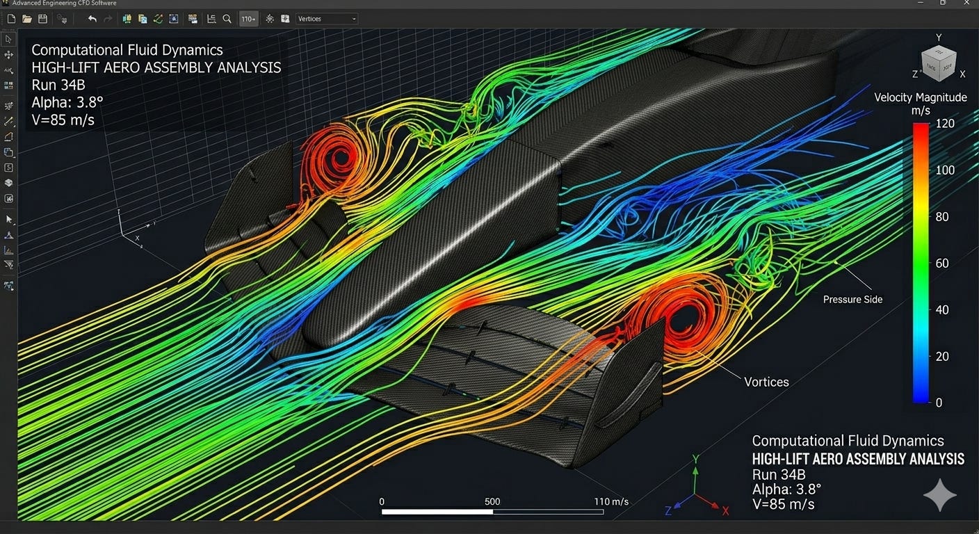
A lot of engineering work is about solving the math of how physical systems behave – for example, stress, heat, airflow, diffusion, vibration. Engineers run simulations (in SolidWorks / ANSYS / COMSOL) to try to turn these real world variables into a solvable numerical problem.
If AI can learn the rules behind this (aka “here’s the geometry, materials, and boundary conditions” and output “here’s what happens”), then iteration gets a lot cheaper and faster. You can explore more of the design space, more often, with fewer specialist bottlenecks. And over time, simulation starts to be embedded inside the design workflow. CAD and CAE begin to blur into one.
One of the most helpful conversations for me around this topic was with my friend Matthew Tamayo-Rios, a PhD student in applied math at ETH Zürich working with Prof. Siddhartha Mishra’s group, which is well known for scientific machine learning (ML for PDEs (Partial Differential Equations) / physics-informed methods).
Below is part one of what I’ve learned since starting to research this space, including some highlights from my conversation with Matthew.
What Is a PINN?
Physics-informed neural networks (PINNs) were introduced in 2017 by Maziar Raissi, Paris Perdikaris, and George Em Karniadakis in a two-part series (Part I and Part II), later consolidated in a 2019 Journal of Computational Physics paper. A PINN is, at its core, an attempt to train a neural network that respects the laws of physics. It’s trained to match the data, but also to respect the physics by adding a penalty to the loss whenever the model violates the PDE. “You want to encode the physics by setting it up as a minimization problem and letting the neural network learn how to solve it,” Matthew told me.
A PINN is basically a function you can query. For example, give it a location inside an object and a time, and it tells you the temperature there. The key is how it’s trained. You’re grading it on two things at once: 1) does it match the measurements you have, and 2) does it obey the basic rules of heat flow, including what has to be true at the boundaries? If it matches the data but breaks the rules, it gets a worse score. Over time, training pushes it toward temperature maps that fit without breaking the laws of physics.
In a traditional simulation, the computer can’t solve the physics at every point inside a solid or fluid, so it breaks the geometry into lots of tiny elements, known as a mesh, and solves the equations at those discrete points. However, meshes are painful because the quality of your answer depends a lot on how you mesh. “Your mesh determines the granularity of your simulation… and in between your mesh nodes, you only have an approximation,” Matthew said. If the mesh is too rough, you miss the sharp, important effects. If it’s too fine, the simulation gets slow and expensive. And if the design changes, you often have to rebuild the mesh and start over.
In a PINN, even though you still have discretized sampling, you don’t need meshes because the neural net is a continuous solution function. The neural net acts like a smooth map you can query at any point. During training, you compute the quantities you need to check the physics for (like rates of change) directly from the model, then penalize it whenever the physics doesn’t balance. The amount by which it fails the equation is the PDE residual.
Why PINNs Seemed So Promising
Most real-world engineering starts with partial signals and a lot of unknowns. You can measure some things, but not all of them (material properties, exact loads, what’s really happening at the boundaries, where the heat is actually coming from, what’s going on between a handful of noisy sensors). You’re basically working backwards from what you can observe to what’s happening underneath.
PINNs let you do physics modeling without needing a ton of labeled datasets. They’re a way to take whatever data you do have and train a model that’s also constrained by the rules of physics. They are often a good way to build approximations when you already know the governing structure and you’re willing to tailor the setup to a specific system. As Matthew put it, they can be “relatively easy to setup as neural surrogates for a specific system.”
That’s why they seemed so promising initially.
Why PINNs Struggle
“PINNs have a bunch of failure modes,” Matthew told me. One big one is that neural nets tend to learn the smooth, easy patterns first, and struggle with the sharp, rapid variations. In other words, they’ll often get the overall shape right but miss certain important details like thin boundary layers or turbulence.
The other issue is that training can be hard. You’re asking the model to do a few things at once: match whatever data you have, follow the governing equation, and satisfy boundary conditions. Those pieces can fight each other. The model can “cheat” by satisfying the easy parts and still getting the physics wrong, especially in stiff or chaotic systems.
That’s why the straightforward version of PINNs aren’t reliably robust enough in the real-world regimes we care about.
Neural Operators: A Shift in Thinking
With neural operators, the idea is that instead of training a model to predict the solution for one specific setup, you try to learn the mapping from a problem description to the full solution. You feed in what defines the problem (e.g. the boundary conditions, the initial conditions, the parameters) and then the model outputs the entire solution field. Matthew’s work is focused here. As he put it, “I’m aiming for a physics-informed operator learning model that is mesh-free.”
Matthew defined “operator learning” as “something that takes any input function or field and maps it to a solution function or field. You give it boundary conditions, initial conditions, and the PDE and it maps it to the e solution over time.” You’re learning the mapping from the setup to the full answer.
One of the best-known examples is the Fourier Neural Operator (FNO). The idea is that it learns the solution operator, which is a mapping from boundary/initial conditions to the full solution, in a way that can transfer across resolutions more gracefully than traditional surrogate models, which are typically tied to a specific mesh or grid. FNO-style models have shown strong results on standard PDE benchmarks, and in some cases a model trained at one resolution can be evaluated at a finer resolution without retraining, aka zero-shot super-resolution.
It’s not a guarantee it will hold in every messy real-world regime and you often don’t truly know the exact parameters of the PDE you’re solving. But it’s the first time this starts to feel like pretraining: “you spend a lot of time training it the first time, and then you can apply it to different types of problems,” Matthew told me.
Foundation Models for Physics
From there, it’s a short jump to foundation models for physics: pretrain over broad families of PDEs or physical systems, then fine-tune for downstream tasks. You see early versions of this in the climate space (for example, ClimaX) and in newer operator-learning efforts aimed at being more general-purpose.
Matthew pointed to Poseidon as one of the early attempts in this direction. “It’s one of the first foundation models that generalizes to unseen physics, and is easy to transfer to new geometries and new parameter regimes.” However, Matthew did caveat this by saying “it still assumes structured grids, requires a ton of data, takes forever to train… and where the physics gets tricky, it starts struggling.”
Those caveats point to the two problems that keep coming up for physics foundation models. First, they demand a huge amount of data, especially in 3D. Matthew’s back-of-the-envelope: sample a 3D volume at 128 points per dimension and you’re already at ~2 million points per time step. Run that over thousands of time steps and the dataset grows very large very fast.
The other big issue is that “in real-world scenarios, you don’t know what the PDE you’re solving is” Matthew told me. You may know the general form, but key parameters are unknown, and it’s unclear which physical regime you’re in. In other words, you’re not just solving for a solution given a PDE. You’re actually trying to solve for a solution given partial physics, unknown coefficients, operating condition ambiguities, and noisy data. That’s what makes deployment so hard.
Put together, these two constraints around data and unknown variables explain why there’s still a gap between research and production. Shipping these models into live environments requires knowing when the models are right, when they’re wrong, and how to calibrate them. It also means embedding these models into the tools engineers already use, which is no small feat in an ecosystem dominated by just a handful of incumbents.
In next week’s post, I’ll explore what it takes to close this gap, which use cases are practical today, and where the ROI is. Trust, calibration loops, workflow ownership, and integration into the tools engineers already use are a few of the topics I plan to cover.
Author’s note: An LLM was used for light copy editing only (spelling, grammar, and clarity). Content, meaning, tone, and structure remain unchanged.