
The Breakeven Point: Rethinking AI for Physics Simulation

Neural networks can solve physical simulations much faster than the numerical solvers engineers have relied on for decades. That is exciting for a lot of reasons, some of which I wrote about previously here.
But neural solvers can be much less accurate than classical ones. And they’re only fast once they’re trained.
In order to train neural solvers, someone has to generate training data (usually by running the very classical solver the model hopes to replace), then train, tune, and validate it. Those costs might be worth it if speed matters. But maybe not.
So when does paying the upfront cost become worth it?
That’s the question Mikhail (Misha) Khodak, together with Yijing Zhang, Nicholas Roberts, and Tanya Marwah, set out to answer in Breakeven Complexity: A New Perspective on Neural Partial Differential Equation Solvers.
Last week, I sat down with Misha, an assistant professor of computer sciences at UW-Madison, where he's been working on specialized foundation models and folding AI tools into algorithm design and scientific computing. In our conversation, we unpacked the research, the motivation behind it, and the impact he hopes it will have on the broader industry.
“It’s not really a case of ‘we’re just going to replace all the classical solvers with deep learning’” he told me, “There are stages of many processes where different things will be useful.”
The pessimism that started it
In 2024 McGreivy and Hakim from Princeton published a paper that landed hard on the field. “They went through many deep learning papers, mostly ones applying deep learning to fluid simulations,” Misha told me. “They found that in a lot of these papers, the comparisons are mainly against fairly weak baselines. The solvers being used aren’t the ones an actual practitioner would use.”
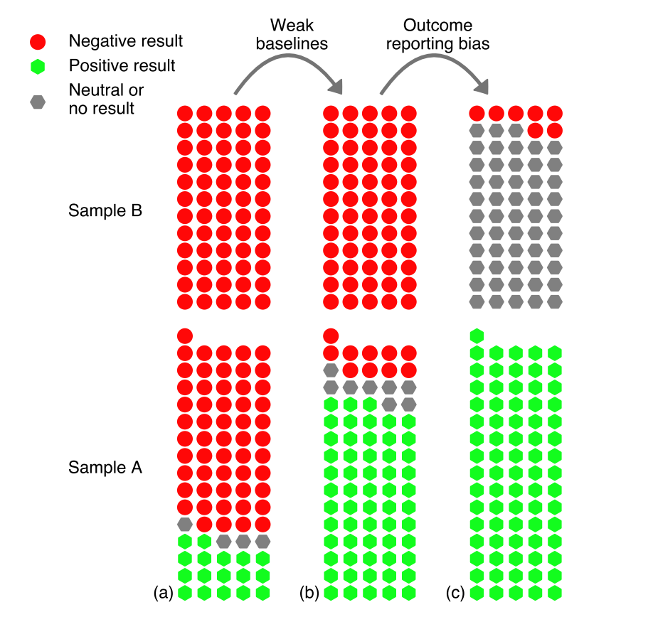
Those papers were overlooking a knob every numerical solver has, which is resolution. You can always make a classical solver faster by down-resolving. “In practice you can set a lower resolution for your solver,” Misha said. “The speed is determined by how many time steps you take and how fine your mesh is. And they often don’t compare to that.”
A neural network that’s “faster” than a high-resolution classical solver, in other words, hasn’t necessarily won anything, because the honest comparison is on speed against a cheap classical solver tuned to the same accuracy.
That paper, Misha said, “caused a lot of pessimism at the time among the scientific computing community.”
Despite the paper, the field kept building. “I was trying to reconcile this issue where we were still developing these ML methods and some people seemed optimistic,” he told me, “but others, especially in the physics community, would tell you to just down-resolve to get a faster solver.”
Counting solves until you break even
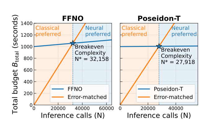
The paper proposes breakeven complexity, a metric that counts the numbers of runs before a learned solver is cost-effective relative to an error-equivalent traditional solver. Error-equivalent here means the classical solver has been down-resolved to the same accuracy as the neural one.
A neural solver only becomes economical when its upfront cost can be amortized. Unlike a classical solver, which pays its computational cost every time you run it, a trained neural network can be reused across every subsequent solve. This is important because most real-world engineering isn’t solving one equation once. As Misha explained it to me, “You are trying to optimize some engineering object. And to do that you have to solve many, many similar partial differential equations.” In practice that means optimizing a design, which requires repeatedly evaluating slightly different geometries, boundary conditions, or material properties. (The paper sets aside real-time applications, where neural networks already have an obvious speed advantage.)
The question then becomes: how many times do you have to run the model before the time you save at inference outweighs the time you spent generating data and training?
The answer, they found, depends a lot on the type of problem you’re solving.
At one end are toy problems, which are simplified academic test cases. “If you want to solve these toy 2D Navier-Stokes with periodic boundary conditions,” Misha said, “you have to perform hundreds of thousands of inference calls before your data generation and optimization cost pays off.” The reason is that for easy problems, the classical solver is very hard to beat even after you degrade its resolution. “For these toy problems there are extremely fast solvers. Even scaling down your resolution, you’ll still end up with a fast solver that is pretty good. So a neural network is just not going to beat it anytime soon. You really need to perform millions of inference calls.”
But as the team moved to harder problems, that changed. As you move to harder problems you require less inference calls in order to make training this neural network worth it. “What happens if instead of Navier-Stokes with periodic boundary conditions you have more regular inlet-outlet boundary conditions, and maybe you throw some blocks in there. Put some obstacles into your fluid flow,” Misha said. “Suddenly that solver becomes very expensive. And scaling down that solver doesn’t just speed it up. The tradeoff becomes much worse. It will be faster but much less accurate.”
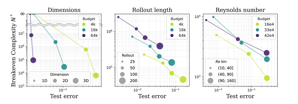
On hard problems, down-resolving the classical solver degrades its accuracy, while the neural network holds its speed advantage at comparable quality. The team confirmed the pattern along several axes of difficulty: scaling a chaotic system from 1D to 2D to 3D, predicting further into the future, and pushing fluids toward turbulence.
Model size and scaling laws for training
Breakeven also depends heavily on which model you use. One of the paper’s more surprising findings is that some of the leading foundation models for physics, such as Poseidon and Walrus, don’t always come out ahead. “In some cases the latest large models are actually too expensive to run, at least on the simulations we tried,” Misha told me. “When I say too expensive, I mean more expensive than a reasonably down-resolved classical solver. So it’s not even worth it to run them.” In several cases, well-tuned, smaller neural operators outperformed the larger transformer-based models, suggesting that “it’s worth it to pre-train very efficient models rather than very large models.”
That same philosophy extends to training itself. Rather than simply throwing more compute at the problem, the team uses scaling laws to determine how a fixed compute budget should be divided between generating training data with expensive classical solvers and training the neural network. As Misha put it, “You can very nicely and consistently predict what is the optimal tradeoff as your computation budget increases.”
Even then, “a practitioner should view this as the upper bound on the performance of a neural network for their problem,” Misha said, “because we are training and testing on the same distribution.” Real-world engineering systems inevitably drift into scenarios the model never saw during training, so neural networks degrade in ways classical solvers generally don’t. Therefore, Misha sees this more as a screening test: if a neural solver can’t outperform a classical solver under these idealized conditions, it’s unlikely to do so in production. If it does clear that bar, it’s probably worth trying on your actual problem.
A funnel, not a replacement
Towards the end of our conversation, I asked Misha what he was most surprised by from this research. “I’m more optimistic now than I was before I started this,” he said. “I actually was maybe more skeptical of neural solvers when I came in. And that’s why I wanted to figure it out.”
Misha also described the future he sees with neural and classical solvers as a pipeline. He referenced the illustration from Periodic Labs, a Zetta portfolio company. “The idea was, with these physical simulations, there’s an agent trying to optimize some material or protein or drug. They’re first going to see what heuristics say is a good candidate, then narrow down. Then they’ll try a neural surrogate and narrow down a bit more. Then they’ll try high-fidelity classical solvers and narrow down a bit more. And then they’ll actually have to go to the lab and build the thing.”
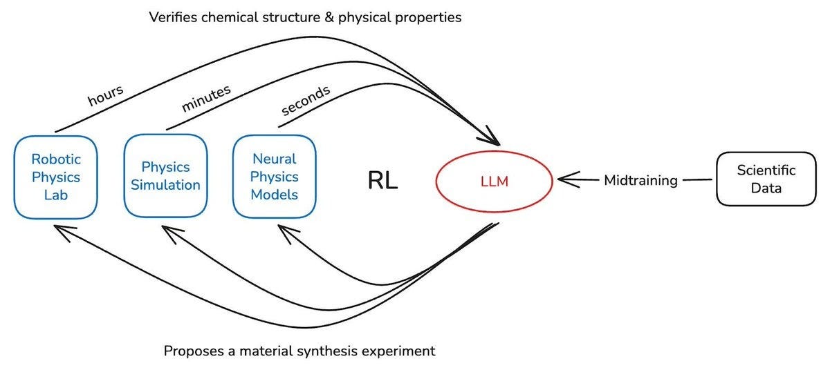
A funnel, in other words where we use cheap heuristics at the wide mouth, fast neural surrogates next, expensive high-fidelity solvers after that, and physical experiment at the narrow end. Each stage tuned to a different point on the speed-accuracy curve.
“There’s room for all of these things,” he said. “It’s not really a case of replacing all the classical solvers with deep learning. There are stages of many processes where different approaches will be useful.”
It’s not a question of whether neural solvers beat the classical way, but rather where each one outperforms vis-a-vis the other. The breakeven paper is the first attempt to answer that question with real numbers.
Author’s note: An LLM was used for light copy editing only (spelling, grammar, and clarity). Content, meaning, tone, and structure remain unchanged.